hyperfine.superconductivity.pippard.specular_profile_dl
- hyperfine.superconductivity.pippard.specular_profile_dl(z: Annotated[float, slice(0, None, None)], T: Annotated[float, slice(0, None, None)], T_c: Annotated[float, slice(0, None, None)], Delta_0: Annotated[float, slice(0, None, None)], lambda_L: Annotated[float, slice(0, None, None)], l: Annotated[float, slice(0, None, None)], xi_0: Annotated[float, slice(0, None, None)], alpha: Annotated[float, slice(0, None, None)] = 1.0, dl: Annotated[float, slice(0, None, None)] = 0.0) float[source]
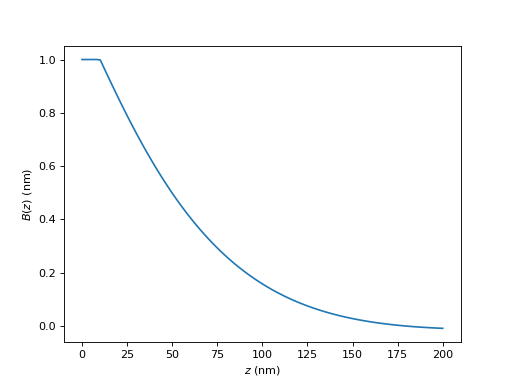
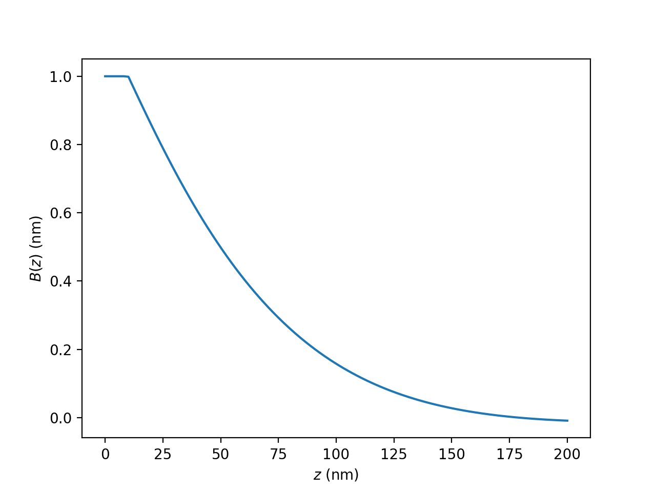
Field screening profile B(z).
The calculation assumes specular scattering of electrons at the material’s surface.
- Parameters:
z – depth (nm).
T – Absolute temperature (K).
T_c – Superconducting transition temperature (K).
Delta_0 – Superconducting gap energy at 0 K (eV).
lambda_L – London penetration depth (nm).
l – electron mean-free-path (nm).
xi_0 – Pippard coherence length at 0 K (nm).
alpha – numerical constant on the order of unity.
dl – non-superconducting dead layer (nm).
- Returns:
The field screening profile B(z).
Example
import numpy as np
import matplotlib.pyplot as plt
from hyperfine.superconductivity import pippard

z = np.linspace(0.0, 200.0, 100)
args = (0.0, 10.0, 1.43e-3, 30.0, 600.0, 300.0, 1.0, 10.0)
b = np.array([pippard.specular_profile_dl(zz, *args) for zz in z])
plt.plot(z, b, "-")
plt.xlabel("$z$ (nm)")
plt.ylabel("$B(z)$ (nm)")
plt.show()
(
Source code,png,hires.png,pdf)