hyperfine.superconductivity.pippard.K_Pippard
- hyperfine.superconductivity.pippard.K_Pippard(q: Annotated[float, slice(0, None, None)], T: Annotated[float, slice(0, None, None)], T_c: Annotated[float, slice(0, None, None)], Delta_0: Annotated[float, slice(0, None, None)], lambda_L: Annotated[float, slice(0, None, None)], l: Annotated[float, slice(0, None, None)], xi_0: Annotated[float, slice(0, None, None)], alpha: Annotated[float, slice(0, None, None)] = 1.0) float[source]
Evaluate the Pippard response function.
- Parameters:
q – wavevector (1/nm).
T – Absolute temperature (K).
T_c – Superconducting transition temperature (K).
Delta_0 – Superconducting gap energy at 0 K (eV).
lambda_L – London penetration depth (nm).
l – electron mean-free-path (nm).
xi_0 – Pippard coherence length at 0 K (nm).
alpha – numerical constant on the order of unity.
- Returns:
The Pippard response function K(q) at q.
Example
import numpy as np
import matplotlib.pyplot as plt
from hyperfine.superconductivity import pippard

q = np.logspace(-4, 4, 200)
args = (0.0, 10.0, 1.43e-3, 30.0, 300.0, 40.0)
k = np.array([pippard.K_Pippard(qq, *args) for qq in q])
plt.plot(q, k, "-")
plt.xlabel("$q$ (nm$^{-1}$)")
plt.ylabel(r"$K_{\mathrm{Pippard}}(q)$ (nm$^{-2}$)")
plt.xscale("log")
plt.yscale("log")
plt.show()
(
Source code,png,hires.png,pdf)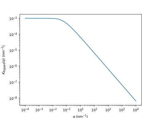