hyperfine.superconductivity.london.GLESolver

class hyperfine.superconductivity.london.GLESolver(x_nodes_min: float = 0.0, x_nodes_max: float = 1000.0, x_nodes_num: int = 1001)[source]

Bases: object

Generalized London Equation (GLE) Solver.

Numerically solve the GLE for a depth-dependent magnetic penetration depth.

See: M. Checchin et al., Appl. Phys. Lett. 117, 032601 (2020). https://doi.org/10.1063/5.0013698

See also Eq. (1) in: M. S. Pamianchi at al., Phys. Rev. B 50, 13659 (1994). https://doi.org/10.1103/PhysRevB.50.13659

_x_nodes: x-values used as the initial mesh by the solver.

_y_guess: y-values used as the guess for the function/derivative by the solver.

_lambda_s: Magnetic penetration depth at the surface (nm).

_lambda_0: Magnetic penetration depth in the bulk (nm).

_delta: Diffusion length of the impurity layer (nm).

_sol: Object encapsulating the solver’s solution.

__init__(x_nodes_min: float = 0.0, x_nodes_max: float = 1000.0, x_nodes_num: int = 1001) → None[source]

Constructor for the GLE Solver.

Parameters:

x_nodes_min – Minimum of the x-values used as the initial mesh by the solver.
x_nodes_max – Maximum of the x-values used as the initial mesh by the solver.
x_nodes_num – Number of x-values used as the initial mesh by the solver.

Methods

`__init__`([x_nodes_min, x_nodes_max, x_nodes_num])	Constructor for the GLE Solver.
`current_density`(z_nm, applied_field_G, ...)	Calculate the current density profile.
`screening_profile`(z_nm, applied_field_G, ...)	Calculate the Meissner screening profile.
`solve`(lambda_s, lambda_0, delta[, ...])	Solve the GLE numerically.

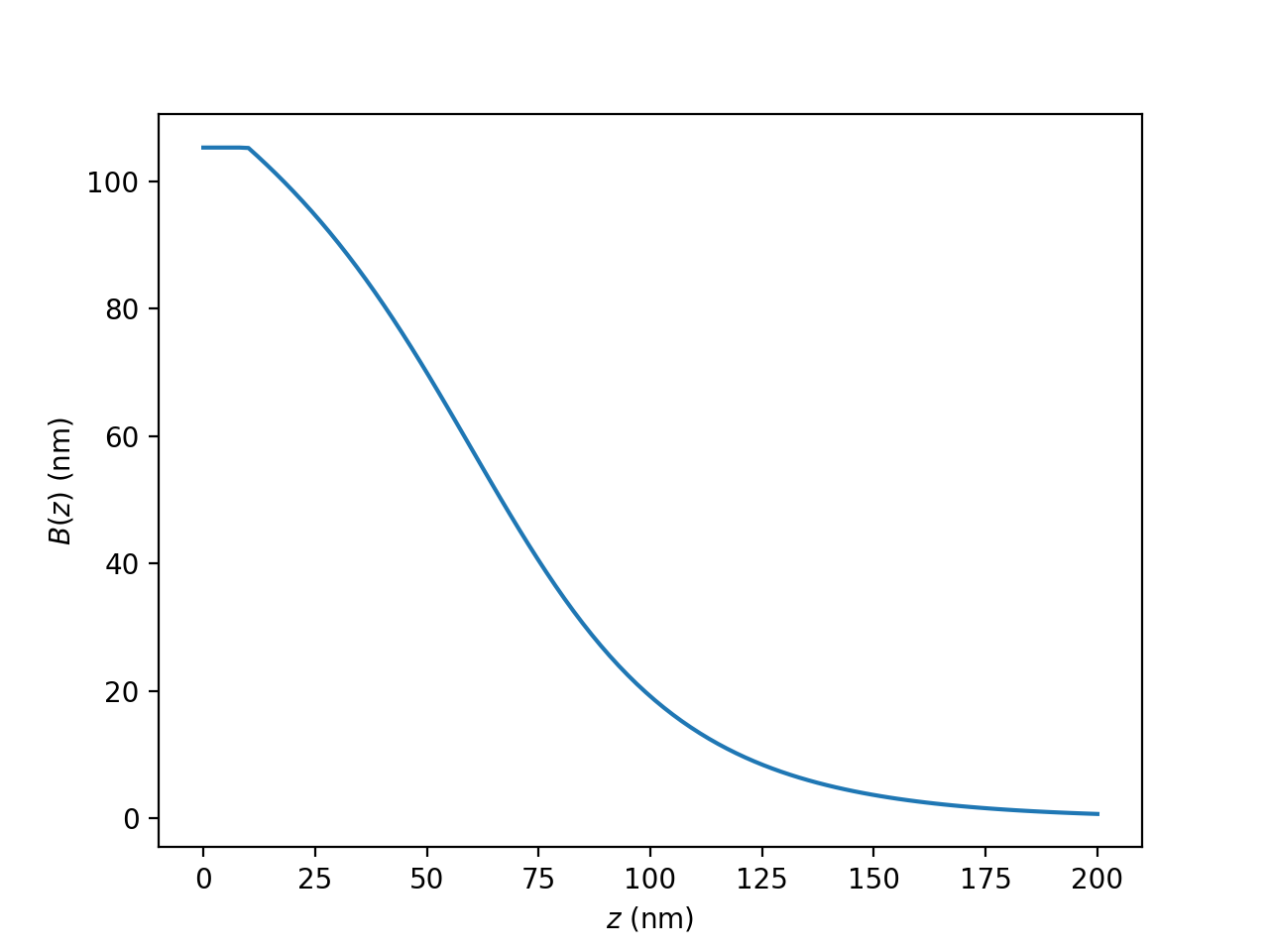
__call__(z_nm: Sequence[float], applied_field_G: Annotated[float, slice(0, None, None)], dead_layer_nm: Annotated[float, slice(0, None, None)], penetration_depth_surface_nm: Annotated[float, slice(0, None, None)], penetration_depth_bulk_nm: Annotated[float, slice(0, None, None)], diffusion_length_nm: Annotated[float, slice(0, None, None)], demagnetization_factor: Annotated[float, slice(0, 1, None)] = 0.0) → Sequence[float][source]

Calculate the Meissner screening profile (alias for self.screening_profile).

Parameters:

z_nm – Depth below the surface (nm).
applied_field_G – Applied magnetic field (G).
dead_layer_nm – Non-superconducting dead layer thickness (nm).
penetration_depth_surface_nm – Magnetic penetration depth at the surface (nm).
penetration_depth_bulk_nm – Magnetic penetration depth in the bulk (nm).
diffusion_length_nm – Diffusion length of the impurity layer (nm).
demagnetization_factor – Effective demagnetization factor.

Returns:

The Meissner screening profile at depth z (G).

Example

import numpy as np
import matplotlib.pyplot as plt
from hyperfine.superconductivity import london

gles = london.GLESolver()
z = np.linspace(0.0, 200.0, 100)
args = (100.0, 10.0, 100.0, 30.0, 50.0, 0.05)
plt.plot(z, gles(z, *args), "-")
plt.xlabel("$z$ (nm)")
plt.ylabel("$B(z)$ (nm)")
plt.show()

(Source code, png, hires.png, pdf)

../_images/hyperfine-superconductivity-london-GLESolver-1.png

__init__(x_nodes_min: float = 0.0, x_nodes_max: float = 1000.0, x_nodes_num: int = 1001) → None[source]

Constructor for the GLE Solver.

Parameters:

x_nodes_min – Minimum of the x-values used as the initial mesh by the solver.
x_nodes_max – Maximum of the x-values used as the initial mesh by the solver.
x_nodes_num – Number of x-values used as the initial mesh by the solver.

_bc(ya: Sequence[float], yb: Sequence[float]) → Sequence[float][source]

Boundary conditions for the solver.

Indexes [0] refer to the function being solved for. Indexes [1] refer to the function’s derivative.

Parameters:

ya – Array of lower bounds.
yb – Array of upper bounds.

Returns:

An array of penalties for the boundary conditions.

_gle_derivs(t: Sequence[float], y: Sequence[float]) → Sequence[float][source]

Right-hand side of the system of equations to solve, re-written as 1st-order expressions.

Indexes [0] refer to the function being solved for. Indexes [1] refer to the function’s derivative.

Parameters:

t – x-values.
y – y-values

Returns:

An array of the system of 1st-order equations to solve.

_lambda(x: Sequence[float], lambda_s: Annotated[float, slice(0, None, None)], lambda_0: Annotated[float, slice(0, None, None)], delta: Annotated[float, slice(0, None, None)]) → Sequence[float][source]

Postulated depth-dependence of the magnetic penetration depth.

See Eq. (1) in: M. Checchin et al., Appl. Phys. Lett. 117, 032601 (2020). https://doi.org/10.1063/5.0013698

Parameters:

x – Depth below the surface (nm).
lambda_s – Magnetic penetration depth at the surface (nm).
lambda_0 – Magnetic penetration depth in the bulk (nm).
delta – Diffusion length of impurities causing depth-dependence (nm).

Returns:

The magnetic penetration depth at depth x (nm).

_lambda_prime(x: Sequence[float], lambda_s: Annotated[float, slice(0, None, None)], lambda_0: Annotated[float, slice(0, None, None)], delta: Annotated[float, slice(0, None, None)]) → Sequence[float][source]

First derivative of the postulated depth-dependence of the magnetic penetration depth.

See Eq. (1) in: M. Checchin et al., Appl. Phys. Lett. 117, 032601 (2020). https://doi.org/10.1063/5.0013698

Parameters:

x – Depth below the surface (nm).
lambda_s – Magnetic penetration depth at the surface (nm).
lambda_0 – Magnetic penetration depth in the bulk (nm).
delta – Diffusion length of impurities causing depth-dependence (nm).

Returns:

The first derivative of the magnetic penetration depth at depth x.

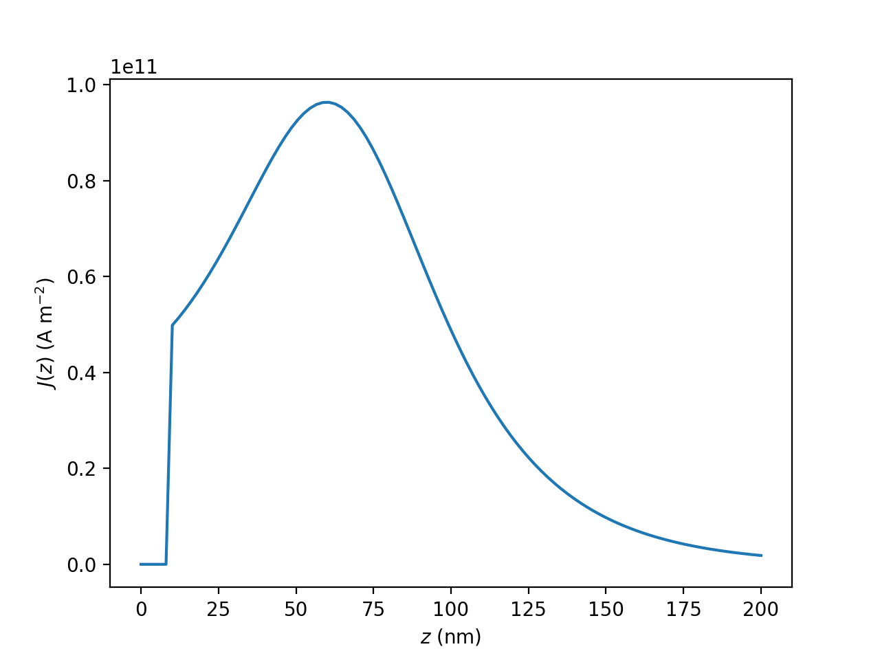
current_density(z_nm: Sequence[float], applied_field_G: Annotated[float, slice(0, None, None)], dead_layer_nm: Annotated[float, slice(0, None, None)], penetration_depth_surface_nm: Annotated[float, slice(0, None, None)], penetration_depth_bulk_nm: Annotated[float, slice(0, None, None)], diffusion_length_nm: Annotated[float, slice(0, None, None)], demagnetization_factor: Annotated[float, slice(0, 1, None)] = 0.0) → Sequence[float][source]

Calculate the current density profile.

Parameters:

z_nm – Depth below the surface (nm).
applied_field_G – Applied magnetic field (G).
dead_layer_nm – Non-superconducting dead layer thickness (nm).
penetration_depth_surface_nm – Magnetic penetration depth at the surface (nm).
penetration_depth_bulk_nm – Magnetic penetration depth in the bulk (nm).
diffusion_length_nm – Diffusion length of the impurity layer (nm).
demagnetization_factor – Effective demagnetization factor.

Returns:

The current density profile at depth z (A m^-2).

Example

import numpy as np
import matplotlib.pyplot as plt
from hyperfine.superconductivity import london

gles = london.GLESolver()
z = np.linspace(0.0, 200.0, 100)
args = (100.0, 10.0, 100.0, 30.0, 50.0, 0.05)
plt.plot(z, gles.current_density(z, *args), "-")
plt.xlabel("$z$ (nm)")
plt.ylabel("$J(z)$ (A m$^{-2}$)")
plt.show()

(Source code, png, hires.png, pdf)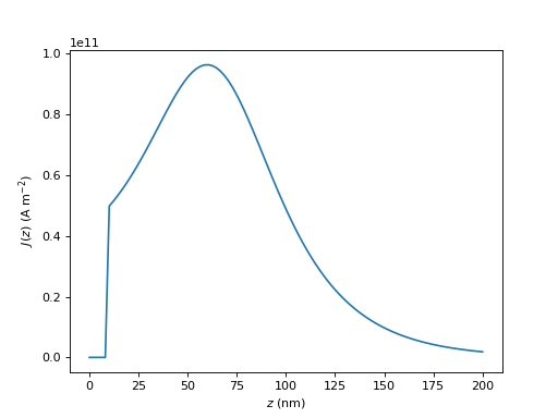

../_images/hyperfine-superconductivity-london-GLESolver-2.png

screening_profile(z_nm: Sequence[float], applied_field_G: Annotated[float, slice(0, None, None)], dead_layer_nm: Annotated[float, slice(0, None, None)], penetration_depth_surface_nm: Annotated[float, slice(0, None, None)], penetration_depth_bulk_nm: Annotated[float, slice(0, None, None)], diffusion_length_nm: Annotated[float, slice(0, None, None)], demagnetization_factor: Annotated[float, slice(0, 1, None)] = 0.0) → Sequence[float][source]

Calculate the Meissner screening profile.

Parameters:

z_nm – Depth below the surface (nm).
applied_field_G – Applied magnetic field (G).
dead_layer_nm – Non-superconducting dead layer thickness (nm).
penetration_depth_surface_nm – Magnetic penetration depth at the surface (nm).
penetration_depth_bulk_nm – Magnetic penetration depth in the bulk (nm).
diffusion_length_nm – Diffusion length of the impurity layer (nm).
demagnetization_factor – Effective demagnetization factor.

Returns:

The Meissner screening profile at depth z (G).

Example

import numpy as np
import matplotlib.pyplot as plt
from hyperfine.superconductivity import london

gles = london.GLESolver()
z = np.linspace(0.0, 200.0, 100)
args = (100.0, 10.0, 100.0, 30.0, 50.0, 0.05)
plt.plot(z, gles.screening_profile(z, *args), "-")
plt.xlabel("$z$ (nm)")
plt.ylabel("$B(z)$ (nm)")
plt.show()

(Source code, png, hires.png, pdf)

../_images/hyperfine-superconductivity-london-GLESolver-3.png

solve(lambda_s: Annotated[float, slice(0, None, None)], lambda_0: Annotated[float, slice(0, None, None)], delta: Annotated[float, slice(0, None, None)], tolerance: float = np.float64(1.4901161193847656e-08), max_x_nodes: int = 2147483647) → None[source]

Solve the GLE numerically.

Parameters:

lambda_s – Magnetic penetration depth at the surface (nm).
lambda_0 – Magnetic penetration depth in the bulk (nm).
delta – Diffusion length of the impurity layer (nm).
tolerance – Convergence criteria for the solver.
max_x_nodes – Maximum number of x nodes used by the solver.