hyperfine.implantation.electronic_stopping.proton_stopping_cross_section4

hyperfine.implantation.electronic_stopping.proton_stopping_cross_section4(T: Sequence[float], A_2: Annotated[float, slice(0, None, None)], A_3: Annotated[float, slice(0, None, None)], A_4: Annotated[float, slice(0, None, None)], A_5: Annotated[float, slice(0, None, None)]) → Sequence[float]

Low-energy proton electronic stopping cross section using four :math:`A_{i}`s.

Empirical Varelas-Biersack parameterization of the proton electronic stopping cross section for scaled energies \(T\) around the stopping power maximum. This version uses four of the five \(A_{i}\)s (\(i = {2,3,4,5}\)) and implicitly determines \(A_{1}\) from them. This alternative parameterization is useful when fitting stopping cross section data without any measurements in the ‘low-energy’ portion (i.e., when \(T < 10\) keV).

See Eqs. (3.1a)-(3.1c) & (3.2) in: https://doi.org/10.1093/jicru_os25.2.18

Parameters:

• T – Scaled projectile energy (keV).

• A_2 – Empirical stopping coefficient \(A_{2}\) (10^-15 eV cm² atom^-1 keV^-0.45).

• A_3 – Empirical stopping coefficient \(A_{3}\) (10^-15 eV cm² atom^-1 keV).

• A_4 – Empirical stopping coefficient \(A_{4}\) (keV).

• A_5 – Empirical stopping coefficient \(A_{5}\) (keV^-1).

Returns:

The proton stopping cross section at scaled energy \(T\) (10^-15 eV cm² atom^-1).

Example

import numpy as np
import matplotlib.pyplot as plt
from hyperfine.implantation.electronic_stopping import proton_stopping_cross_section4

A = (6.73, 1.03e4, 2.8e2, 3.9e-3)
T = np.logspace(0, 4, 200)
S_e = proton_stopping_cross_section4(T, *A)

plt.plot(T, S_e, "-")
plt.xlabel("$T$ (keV)")
plt.ylabel("$S_{e}$ ($10^{-15}$ eV cm$^{2}$ atom$^{-1}$)")
plt.xscale("log")
plt.show()

(Source code, png, hires.png, pdf)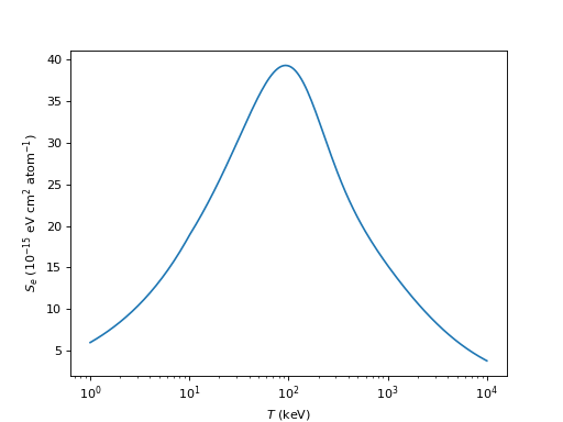